Project 4 Week 3: Finding Optimal Routes for Wine Delivery

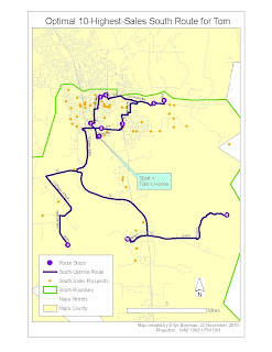
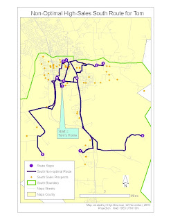
This week we looked at the same three wine sales territories in Napa County and used Network Analyst to find the best route - NA can do this by time, using a field for speed limit for each road segment, or by miles, which is how we did it - for a sales representative in each territory, starting from the sales rep's home. For this particular exercise we selected the top 10 sales in each territory, created a list of sales stops from these 10 (using Network Analyst), and then created a route, again using Network Analyst, that takes the sales rep from the home starting point to all the 10 stops.
Interestingly, the default route is based on the number of the OBJECTID field in the sales prospects attribute table, rather than any other geographically-related field, so this route is likely to be a) long and b) nonsensical: for an entertaining example of this, see the map on the right (the Non-Optimal one for the South territory). If you look closely at the numbers to see the order of stops, you can see how little sense it makes.

As I mentioned above, however, Network Analyst does have a setting that allows you to create an "optimal" route, in this example the one with the smallest number of miles to cover: see the map on the left. It also allows you to print out a set of directions from to get you from designated stop to designated stop. You will note though that many stops near the 10-highest-sales ones are not included in this example. Left unaddressed is who is going to trail along and pick up the slack using another, less lucrative route!

We could have symbolized the roads in these maps according to the prevailing format - freeways in 3.4 width red, lesser highways in black with the usual symbol, etc. - but the important thing in this map is really the route the sales rep is supposed to follow. Hence I chose to leave the non-route routes in pale grey regardless of their size, and the route roads are the only ones I labeled since they are the ones that the sales rep is looking for. If I were the sales rep I would also throw a good, large-scale county map into the car/truck, just as insurance: ArcGIS directions are only as good as the data, and we know that Google directions, which are generally pretty good and which probably come from very similar data, can slip up royally from time to time.

Related to this is the fact that one of the sales stops on the original map for the Northeast territory could not be located by Network Analyst. It appears that the road on which it sits does exist, but it wasn't in the road network dataset that we used. So the stop was located correctly, but Network Analyst couldn't figure out how to get there because it couldn't see the road. I tried to move the sales stop point to the nearest road, but ran into immediate difficulties as when I reran the route calculations, nearly half of the sales spots showed up as not located. So I took the easy route, so to speak, and dropped the problematic sales stop in favor of the one next on the sales list. If I had a bit more familiarity with NA I expect I could have fixed this, but Project 5 is looming and it's Tuesday already.

Project 4 Week 2: Assigning Delivery Areas for Wine Customers

This week we had to divide Napa County into three parts. three ways. First we divided the number of wine customers (290) and their sales. The first slicing of the county (no name attached) was by number of customers and sales: each third on the map had to include 95-97 customers and 1/3 of the total county wine sales, +-5%. The next, called Territory 1, was just a straight geographic division, using straight lines (they all intersected near the densely-populated south-central portion of hte county. The final slicing (called Territory 2) attempted to divide the county using roads as the boundaries, preferably major roads. I had to use one minor road for this. A link to the resulting powerpoint is attached: http://students.uwf.edu/db27/BayArea/Week2WineDeliverable.ppt

and above is a graphic just for the sake of decoration: (this is the first one, equal sales and equal numbers of vendors):

One of the interesting things about this was how little tweaking is needed to change the figures considerably and skew the sales over to one section or another, because of the density of stores and restaurants in the south-central region. My territories 1 and 2 didn't do a great job of equalizing customers and sales, although it's clear that it wouldn't be hard to do that. A more thorny issue is that the South area, under the current criteria (number of customers and total sales potential), benefits unfairly because deliveries would take a lot less time given how close the markets are to one another.



I had a fair amount of trouble with this one because I missed a note about the need to edit the "Territory" column (to reapportion areas from Northwest to Northeast, or South to Northwest, or whatever) after each new set of boundaries was created. Eventually I figured that out, but there were a couple of "ghost" points - one because it fell outside the Napa County shapefile boundary line, another for no reason that I could see - that were also confusing. I am getting better at editing things in ArcMap though, which is a relief. This week also did bring home how useful it must be to be competent in programming, to avoid having to do the same thing over and over and over and over...

Project 4, week 1: Wine Sales in Napa County

This project is about transportation routes generally, for wine sales in Napa County, California specifically. We created maps of population (well, numbers of households) as well as of liquor, restaurant and wine sales, with the distribution of restaurant and liquor stores superimposed on these maps.
This was a pretty straightforward week. I look forward to learning a bit more about using Network Analyst - I have created networks in ArcView (pre-ArcGIS) but haven't managed to do anything in 9.0 or later.
The link to the pdf which contains these maps: http://students.uwf.edu/db27/BayArea/NapaWineMarket.pdf

Week 9: reporting on the best spot for a bookstore

The mechanics of this week were fairly straightforward although the numbers - on which we would hypothetically be deciding to site a bookshop - were rather less so; one could make legitimate arguments for more than one possible location. I recalculated figures for each site using the census blocks that had their centroid within the 1-mile radius around each location. This is something that I really appreciate about GIS, the ability to summon the location-based figures so rapidly. Here's the powerpoint link for the final report:

http://students.uwf.edu/db27/BayArea/FindingANewLocation.ppt

week 8: choosing a store site in San Francisco

This week we looked at two more ways of defining market area: by the sales figures within a radius around the store, and by drive time to the store. In fact if one was looking at a potential store site in downtown San Francisco, drive time may be less relevant because - especially for something like bookstores, and in a city that is as walkable as San Francisco - probably a significant proportion of buyers are walking to the store. However "drive time" could be altered to walking time without much difficulty.

So far the assignment is pretty straightforward, although I can see that determining the best store site is going to be tricky because each potential site is good in some important areas (e.g. high population growth) but bad in others (e.g. lower household income).

This week two maps were the products. One shows market area measured by drive time and by the proportion of store sales. The other shows the location of potential available stores as well as the location of current competitors.

Week 7? Project 3 Prepare: Market Analysis, Site Selection

The multisectioned map above shows the San Francisco area with two storefronts of the hypothetical Better Books business, and various demographic aspects (household income, percent with some college, etc.) of the area. The one-part map on the left shows average house value (for my own interest) but it also indicates a one-mile buffer around each of the stores, which is presumed to be the market area. This week's work was relatively uncomplicated one. In some ways the tables I created (not shown) to go along with the maps were more interesting, because they showed a smaller overall dollar intake from the Steiner market area but a considerably higher average purchase for each Steiner Book Lover customer. Nice to know that it's not always maps that are illuminating.

An unrelated but useful map-related thing I learned this week - for my internship work, not for this - was that cutting down the size of your data can make a big difference. In my case it was the difference between having ArcGIS run and having ArcGIS freeze, so I was pretty thrilled when I finally figured it out. The dataset in question was a huge watershed file. It was a big advance when I realized that even though I could use a definition query to reduce the size of the visible file, that wouldn't stop my freezing problem. Selecting and exporting part of the data file made an astonishing difference. Next time I have big files I hope I remember to spend a small amount of useful time at the beginning to avoid spending a lot of unproductive time later.

Week 6: Saving Energy via Trees

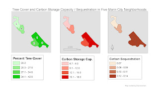
For this , the report week of the landscape design section, we had first to calculate the energy savings produced from planting trees in our study area. This was more a mathematical than a GIS exercise (once we had the proportion of Marin City, or several Marin City neighborhoods) that was covered by trees. For the second part, we had to determine how many trees would be needed to offset the anticipated energy demands of a new Marin City Center (its area outlined in yellow on the map). This was based on a combination of a) the area covered (calculated with GIS), b) the average monthly electricity usage of a commercial building (from a Department of Energy table), c) the annual energy savings produced by one tree (from another table) and d) the previously-calculated (maximum) number of trees that could be put on the site. It is interesting to see how GIS can intersect with this type of work, and also interesting to see how much of the input is tentative, or at least hypothetical - we don't know whether the average tree's energy savings will be the same as our Marin City average tree, for instance. Still, interesting to do.

Week5: Carbon Sequestration and Tree Cover

This week we had to calculate tree cover from our previous week's raster creation. Last week we had to generalize a raster that was classified into 50 classes (or 25 if ArcMap kept crashing), and generalize it to 3 classes: trees, grass and impervious surfaces. (So that's how it's done!) This week we calculated the area of the tree cover as a percent of the whole, and also did some carbon sequestration calculations. The three resulting maps (shown here) are quite similar. The 2nd and 3rd display, carbon storage and carbon sequestration, are really the same thing multiplied by a different constant.

This week I learned more (than I wanted to know, really) about the Field Calculator, but it was useful. I also discovered how to join the five neighbhorhoods that we focused on, using the Append function. That was useful too.

Last week we had the task of joining 7 smaller rasters into one big file. This didn't go at all well for me until Mari suggested using mosaicking, a technique I had never used before but that was very useful and worked like a charm.

All in all things are going pretty well. Except for the eyestrain this week...

Week 3: Mapping Proximity to Target Population and Asthma Triggers

For the final week of this asthma-related project we had to do a proximity analysis to show which Alameda county hospitals were a) close to census tracts with a high proportion of black residents, the target population (I used more-than-50%-black; most of the census tracts were near South Berkeley and in Oakland), b) close to major roads (buffered by 0.1 mile), and c) close to Toxic Release Inventory (TRI) facilities (buffered by 0.5 miles). All went fairly well until I got to the point of doing Euclidean Distance for each of the inputs (hospitals, high-black-pop, TRI and roads). First I made at least 20 tries to endeavor to figure out which of the "environments" and "analysis" settings for the Euclidean Distance function did what. Eventually I discovered the distance between a mask, which could be the shape of a shapefile if needed, and the raster analysis extent, which is a rectangle. (Perhaps I was told this earlier - but if so, I had forgotten.) I also discovered that if you set the analysis extent to "extent of display", and adjust the display, the distance radii become longer or shorter. It was an instructive, if frustrating, process. I was pretty excited when I finally got it straight, but it was a long road to enlightenment.

Perhaps I shouldn't have shown this map, since it makes glaringly obvious the difference between the outline of the Alameda County boundary shapefile (the western part, where I did the analysis, is in color) and the outline of the Alameda County census tract shapefile (that grey thing sticking out at the bottom is a high-black-percent census tract that extends beyond the Alameda County boundary shapefile that I intersected with the analysis extent). However it does show the areas where the hospitals are close to a combination of high black population, major roads, and TRI facilities (closest hospitals are in the lightest yellow section). I made the black population file the most important (worth 60%) when I did the weighted overlay of the four files (hospitals (10%), TRI (15%), roads (15%) and black population) because the most important thing is for the hospitals to be close to where the target population is.

Fall Week 1: Preparing Data for GIS & Public Health

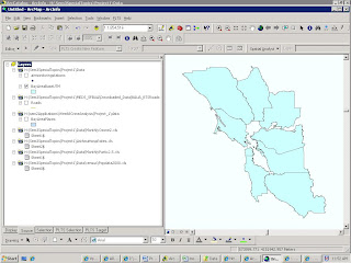
In this first 3-week section, we will be producing maps of Bay Area demographics as well as asthma hospitalization rates and some pollution indices. As part of the preparation, we had to compile a metadata chart containing the layers we would need to use. I can't for the life of me figure out how to link it to this, so instead here (to the left) is a screen shot of the layers I plan to use; below is a link to the same thing, only bigger.

http://students.uwf.edu/db27/BayArea/Week1ScrShot.jpg

I haven't included anything in this screenshot other than the outlines of the Bay Area counties. I'm still having some problems, with a) having a correct, or complete, roads file - although the roads aren't crucial for the public health part, I think, so far; and b) with the correct projection for the air sampling stations, which so far has eluded me. Maybe by next week...

Week 5: Using LiDAR

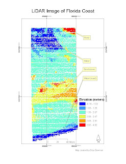
This week we learned how to import a .txt file of raw LiDAR point data into ArcMap, convert the data into a raster image in ArcMap and transfer that image back into ERDAS. This wasn't so hard; the difficult parts for me in the challenge part of the lab were

a) figuring out the scale (until I read the .xml metadata file and realized what the projection was I kept getting impossibly small figures for the scale),

b) wondering where on earth I was - when I was still confused about the scale I did discover - by checking the coordinates into Google Earth - that the location must be the Florida coast again and not in the middle of Iran as I thought for a perplexed moment! - and

c) 'reading' the raster image to figure out which was road and which was sand dune. The road, I concluded, was the part at the top right (it shows up in red in this image) with fairly uniform elevation and a longish straight side, but it took a while before my different classifications showed that. I think I got it eventually - it was initially hard to see. With the manual classification I did (I chose not to use a "stretched" continuum of color) I found it easier to find the road. I ended up creating a rather luridly colored image but water shows up clearly, here as blue (because the elevation is near zero) and sand dunes are yellow and orange. The whole process did reinforce for me what a rube I am when it comes to remote sensing. If only I'd taken a full semester of it when I had the opportunity!

Week 4: Supervised Classification

Here is a link to the map that resulted from this week's lab: http://students.uwf.edu/db27/RemoteSensg/Week4.xps
I'm finding RS really interesting even though the software is dismayingly unfriendly to the user (but powerful). This week we classified land cover types from a satellite image, and then recoded some of the land cover types (merging classes to make fewer classes). I had trouble with recoding in the challenge lab although it seemed to go OK in the main lab. Still have questions about the mechanics of this - remote labs are OK but the discussion board for questions works only so far. I'm finding ERDAS to be a sort of Frankensteiny monster - powerful but lurching from side to side unpredictably (not to mention crashing without warning) and so far it's awfullly hard to get it to do what I want. More practice would help. I wish I'd taken remote sensing when I did my geography degree and was actually present in person!

Week 3: Orthorectification

This week we placed control points on images and tried to orthorectify the images by making reference to a topo map (or, in the first part of the lab, to specific points on an image). This was an interesting experience that I was able to repeat many times because of the program crashing repeatedly. I understand the general idea but I had a lot of problems with the software, which makes ArcGIS look like a walk in the park.
The final image is the orthorectified one, with a UTM map grid superimposed. I am not sure whether it is clear that the final image has been orthorectified. I think the software does a lot of useful things, but it currently has some built-in frustrations.
A link to my orthorectified image is at http://students.uwf.edu/db27/RemoteSensg/Week3PensaRectify.xps

Week2: Discerning Differences Using Spectral Bands

This week we looked at an image taken near Puget Sound, Washington and examined the image information, including the pixel histogram and the pixel data, for specific places in the image where pixel values in certain bands were particularly low or high. I still find ERDAS Imagine a frustrating and non-intuitive form of software, but in looking at the image using different wavelength bands I was captivated by the scope for interpretation and visualization. This made it a really interesting lab (when I was not cursing ERDAS). I still have no idea where Map Composer is or whether it (or its logo) even exists within the software, but I did eventually find all the pieces of things I needed to finish the lab.
Links to my images:
http://students.uwf.edu/db27/RemoteSensg/Week2Layout1.xps
http://students.uwf.edu/db27/RemoteSensg/Week2Layout2.xpshttp://students.uwf.edu/db27/RemoteSensg/Week2Layout3.xps

Week 7: Location Decisions, Our Choice

Not sure if a blog is required this week so am forging away. This week required the same work as last week, but the criteria and the location were our choice. I briefly considered Durham, NC, but I can't easily get the shapefiles I would like - FGDL.org has a better centralized shapefile inventory than the NC equivalent or than what I could get from Durham. I chose Leon County, NC, largely because it had an interesting rail-trail and a university, Florida State, in Tallahassee. I wanted a location that was close to libraries, to FSU, and to the rail-trail, but also with high median house values.

This provided an interesting conflict because central Tallahassee has low house values (and correspondingly high poverty levels), although this area is close to the uni and near public libraries and the trail. So the result is a tradeoff: which is more desirable: high house values, or the amenities that make life worth living?

I've attached my poster, or at least what I think is a poster, detailing the process and the outcomes.

Remote Sensing: Week 1 maphttp://students.uwf.edu/db27/Pensacola1.xps

http://students.uwf.edu/db27/Pensacola1.xps
The map to which this link should direct you is my first map in ERDAS (ERDAS IMAGINE 2010, which looks like the latest Windows interface, alas). It was an interesting - perhaps frustrating would be a better word - experience, but at least it was a learning experience. I'd like to know more about in what way ERDAS is better suited to displaying aerial photographs, etc. than ArcGIS (after all that time I have spent making sense of ArcGIS!) I hope it will get easier with practice.

Final Carto Project: SAT Scores

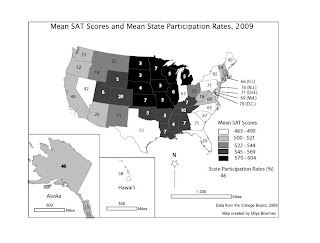
The caption for this map is

State mean SAT scores and SAT participation rates. In general, as a greater proportion of a state's high school graduates take the SAT, the state mean SAT scores fall, and vice versa.

This map was our final project. We were given a link to a table with either ACT scores or SAT scores, and state participation rates. We had to pick SAT or ACT, create the map from the data, and include both scores and state participation rates. I typed the data into an Excel file, joined the Excel file to a state boundary file in ArcMap, and once I had symbolized the mean SAT scores on a choropleth map, exported it as an Adobe Illustrator file so I could position the state participation data as numbers on each state.

Initially I downloaded from the web a free, recent TIGER census state boundary file to join to the SAT data. This worked really well right up until the point in Adobe Illustrator when I was almost finished with adding the participation rates and discovered that Michigan was unrecognizable because the TIGER folk had generalized the state's boundaries to include (i.e. to swallow) Lake Michigan. Concluding that the average newspaper reader would be confused too, I discarded the map and after some unsuccessful web searches, hunted down an ESRI shapefile at my local university's (UNC-Chapel Hill) GIS data depository.

The process for this project was fairly straightforward. I am least pleased with the size of Alaska. I wanted everything to the same scale, and I know it is supposed to be bigger than Texas and California (and a few other states) combined, but I now think the map would have been improved if I had scaled Alaska down a bit to match the size of the rectangle around Hawai'i. I put Hawai'i and Alaska in separate data frames so I could manipulate them into the same layout; I tried to exclude them on the main data frame with a definition query but failed, so I moved the mainland on the screen to remove them instead.

This map is an interesting example of how data left out can mislead. Without the state participation rates, one might understandably assume that for some reason the high school students on the east coast were dullards and those in the midwest and south - except for Texas - were a bright bunch, or at least had better education through high school. Adding participation rates is clearly an improvement, although more information overall would be useful so we might know just who writes the SAT in each state and how they compare with those in other states.

Week 11: Using Google Earth

This week our task was to locate a suitable site for a wind farm somewhere in Ohio and then put a placemark at that spot in Google Earth. We were given links to information about criteria for suitable sites, and links to some maps.

Fundamentally, the wind turbine site has to have a minimal average wind speed. Additional criteria mentioned on the BERR website include landscape and visual impact (related to tourism though not entirely), ornithology (Bird migration patterns), noise (related to distance from dwellings), shadow flicker (ditto), and shipping impact (here, around the Great Lakes).

I started by downloading a wind map. I first found the 80m wind power map of Ohio produced by the US Department of Energy’s National Renewable Energy Laboratory. Later I found a 50m version (better resolution) of the same map, also by the NREL, dated 2004. In addition, the summary report by the Health Assessment Section of the state’s Bureau of Environmental Health (March 2008) notes that the “best areas for utility-scale wind turbines are Lake Erie off-shore, the Lake Erie shoreline, and topographically-elevated portions of….Logan, Champaign, and Hardin Counties” (p. 2).

After looking at maps of the Great Lakes shipping routes and at another map of Ohio state parks, many of which are along the Lake Erie shoreline, I decided that siting wind turbines in Lake Erie was likely to be problematic not only for shipping but for tourism reasons – there would also be considerable recreational boating in the area - and wind turbines here would therefore probably be subject to considerable opposition. I returned to Logan, Champaign and Hardin counties.

Next I pasted together three small printed maps of census 2000 block group population, one for each of these three counties: I got the information from the FactFinder section of the census.gov website, which allows you to map a variety of demographic characteristics, including population, down to the block group level, and which I have found very helpful in the past. This gave me a general idea of areas to avoid: in each of these counties there is a population concentration more or less in the center of the county.
On to the pasted-together county maps I did a sketch of the areas on the NREL map that had the highest wind power classification (6.4 – 7.0 m/s at 50 m).

I consulted the npwrc.usgs.gov website about migratory patterns of birds, but those were so general that all I could tell was that some birds would be migrating across this section of Ohio.

USGS.gov has downloadable topographic maps, which would have helped to determine the hillier areas in the counties, but unfortunately the maps are so tiny for the amount of detail on them that it is almost impossible to determine where the high elevations are. I did conclude that it would be better to have the wind turbines on the west or southwest side of hills, partly because the wind will be coming from that direction and partly because there will be more shade to the north of the turbines; but I am not confident that my final choice is actually on a hill because I couldn’t make out the topography in Google Earth or on the downloadable topo maps - I don't have the experience using Google Earth to make out hills, and I don't think Ohio has many hills that are too steep for growing crops in regularly-shaped fields..

I also checked a map of state parks. Many of these are on the Lake Erie coast, as mentioned, but there is also one in Logan and one in Champaign county, each of them in the northwest portion of the county. The wind power areas from the NREL map were chiefly in eastern and northeastern Champaign county, in eastern Logan county, and in a couple of spots to the south and west of Hardin county.

My final site is in southern Hardin County, a little north of the border with Logan county. It is in a rural area, not close to any parks or any large population centers. I think this section is a bit higher - at least it's supposed to have higher wind speed - but I can't be certain. The problem with dealing with Google Earth and GIS maps - at least in this instance - is that although the resolution of Google Earth is very good, we don't have the other, lower-resolution GIS data superimposed on it, so at least in my case, the final wind farm site may not be in the best spot. I'm hoping the people who actually make these decisions do have integrated data! I do think Google Earth is a fabulous tool and has marvellously specific resolution which I have used on a number of occasions, and I know there will be other interesting things to do with it in the future.

Week 10: Contour maps

This week we had to draw contour lines - they are for yearly precipitation for the state of Georgia - on a map in Adobe Illustrator. First we had to draw the contour lines by hand, using a paper map that had point data from dozens of spots, about one per county (Georgia, it turns out, has 159 counties). We had to interpolate the point data manually, eyeballing the lines from point to point, in order to create the contour lines. Then we were to transfer the lines from the printed map to the map in Adobe Illustrator.

I thought the process of creating the contour lines was tremendously interesting, as well as a challenge, especially where the data went down and then up and down again - since rainfall inconveniently does not go smoothly in one direction up (or down) across the state. I found myself resorting to a beautiful 1970s book of maps of British Columbia for a better look at how one deals with the ins and outs of contour lines; this in turn reminded me pleasantly that I've been fascinated by maps for a really long time.

As usual, Adobe Illustrator provided its own set of challenges. I had hoped to color the spaces in between the lines, but my technical skills in Illustrator aren't yet up to the job and I gave up after I got the easy parts (the closed loops) done. The map still has problems. I made a mistake somewhere and couldn't correct it: even after selecting every one of the 159 counties and clicking on the "stroke" icon to correct the county outlines, I was unable to get several counties to match the rest exactly in outline color: you can see this at the south end of the state. But it is recognizably Georgia! and the contour lines are there, so that's how it stands.

Week 9: Flow Maps

For this week's lab we had to take a world map in ArcGIS, decide on its projection, and transfer the map to Adobe Illustrator to add flow arrows showing the number of people gaining legal permanent residence in the U.S. in 2007 from each continent.

After printing and rejecting several projections, I decided on Buckminster Fuller's icosahedral one (similar to gnomonic apparently) because it preserves shape well and the continents weren't tremendously distorted in size, and because I've always been intrigued by Fuller and this was my first opportunity to use an invention of his! It did however complicate my north arrow positioning, with which ArcMap did not help me. I am afraid that the north arrow in Illustrator is the result of me blindly aiming for the North Pole.

This time I found the Illustrator videos were quite helpful - having the narrator not rush the words made a big difference. As for the data, I separated arrows for Canada from the flow from the rest of North America because they were coming from two different directions. I chose not to include the GIS file of all the individual U.S. states, since I thought they would only clutter a map that does not display which states are the particular destinations of immigrants.

Dot Density Maps

This week we had to take some Florida population / housing unit / land area data, in Excel calculate housing density (I used housing units per land area rather than per total area) and create a map of housing density, using Adobe Illustrator again.

I ended up creating two maps because we had a lot of confusion about which we should be doing, raw housing unit (or population) data versus density (units per area). I wanted to see how different the maps would look. In the end I haven't really answered this question well because in the density map for some reason I didn't position the dots as randomly as in the housing units map. The dots in the housing units map are also very slightly larger than those in the density map - 0.8 pixels instead of 0.7 pixels each. I had tried selecting all the dots and then transforming them "Each", but when I did this with large transformations the dots moved as well as expanding/contracting, so I haven't really solved this problem. Overall the maps look quite similar in terms of county-to-county relative amounts of dots, despite differing distributions from map to map within the individual counties.

I feel more comfortable with the housing units map, or at least with the idea of mapping raw data with dots rather than density with dots, but I could see mapping density at the county level if the data were census tracts or something finer than county level. I would like to try this exercise out in ArcMap. I haven't yet learned how to make a template (assuming this is possible) in Illustrator, which may be why not all of my map pieces are identical - the north arrow is in a slightly different place in each, for instance.

Other than that and my gradual lessening of alarm while in Illustrator, I learned how to make a north star a la the cartography text, which pleased me.

Week 7: using proportional symbols

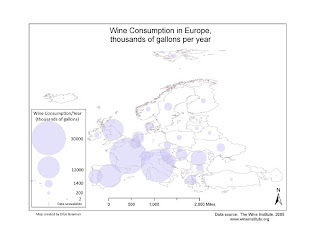
This week we had to take a simple map of European countries in ArcMap and export it to Adobe Illustrator so we could add proportional symbols in Illustrator. The data came from an Excel file of wine consumption for each country. We had to convert the figures for wine consumption using the formula for representing values via circles (it involves square roots), and represent each country's wine consumption with a circle of the appropriate size.

This went pretty well, a bit to my astonishment but now I have a better idea of how to organize my layers and am a bit more likely to be able to undo unintended errors. In Adobe I did have two peculiar unwanted rectangles that refused to be selected (and hence, to go away), but fortunately they disappeared from the final map when I exported it to a .jpeg. Next time we do something in Adobe Illustrator I'll try making a decent north arrow. If I had more time I'd put the Excel info into ArcMap and see how different that map looked, but I feel pressed for time. I still feel a bit at sea in Illustrator, although I think I can spy land.

Week 6: Using Adobe Illustrator to make cloropleth maps

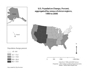
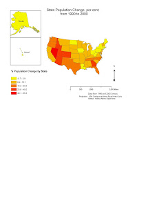
For this week's assignment we first had to create a simple color cloropleth map of population change state by state in the U.S., open the map in Adobe Illustrator and make a few more changes as needed. This went reasonably well until the Illustrator part, although I also had problems with projection because we had to include Hawaii and Alaska on the map. Eventually I put Alaska in a different data frame (and different projection). The map ended up having about three different data frames and I had trouble arranging them all.

For the second, grayscale, map, we had to open an Excel file of the 1990 and 2000 population figures for each state, calculate the percent change in population for each state, and aggregate the data into averages for each of the regional census divisions (there are 9 of these). The range of values for this second map had to be categorized on an equal interval scale, unlike the color map (map #1), the data for which was categorized according to natural breaks. Then we had to open the first map in Adobe Illustrator, convert the colors for each state to grayscale, and assign the correct color on the grayscale scale to each state, according to where it sat in the census division region. This tinkering also included redoing the numbers for the legend. This wasn't quite as bad as I thought it wuold be, as I am now figuring out how to organize layers and objects in Illustrator, more or less.

Only map #2 (grayscale) is in landscape format, but #1 will have to stay in portrait orientation for now, as I only managed to save the file for #1 in the right format when I was halfway through the changes to the map to make it into #2!

Week 5: South/Central Florida's Hispanic Population, in Adobe Illustrator

This week's assignment was to take a ready-made map in Adobe Illustrator and rearrange the items so that the information was displayed better. We also had to add a north arrow and a neatline. You can see the original on the far left; the one on the right is mine after my changes.

I had a lot of trouble with this assignment and I'm not perfectly satisfied with the end result, though I do think it is an improvement. It took me ages to get the legend in the right place relative to the south/central map of counties. I admit I did not see the videos before getting the map done as I kept getting error messages when I tried (in fact AFTER uploading the final image to this blog I tried one more time and lo and behold, this time the first video worked) - I have been consulting a book on Adobe (and various Help messages on their website) .

I removed the extra zeroes that were originally in the legend percent figures, as they are statistically meaningless as well as confusing to the reader. I used the Kuler tool to find a "swatch" of five colors, but I could not find a Kuler swatch that simply went from light to dark and the one that was closest to what I wanted had two reds that I could not distinguish once they were on the map, so I changed one of the colors in the five-color range to make the differences clearer.

I didn't like any of the arrows that Adobe offers - importing a graceful one would be better - so I compromised by thinning one of their arrows once it was on the screen. I couldn't do anything about the scale bar, which looks too big and clumsy - and is now equidistant from the small-scale and the large-scale Florida map - but I had to let it stand. Maybe when I have better skills I'll be able to fix that! In a word - Phew. I'm glad to have this lab over.

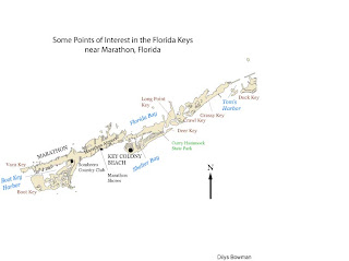
Week 4: Using Adobe Illustrator in labeling a map

This is my first stab at Adobe Illustrator. The assignment was to label this map of part of the Florida Keys: we were to label four bodies of water, three parks or city features (a country club, a state park and an airport), three cities or towns, and seven islands (keys).

Apart from the frustration of using a new program for the first time and my inability to separate parts of the drawing from other parts (so that I could fill the state park in in green, which you see I have not managed to do), my main dilemma was how to represent things. In particular, the map is absent a legend because there is essentially nothing symbolized. I fear this may come back to haunt me. I did choose to represent the labels with different colors to separate park from water body from island(key).

I have the feeling that there's a lot about Adobe Illustrator that would be very useful, though I don't feel competent enough to enjoy its capacities yet.

Data classification methods: percent black population in Escambia County, Florida

This week we used Census 2000 population data for Escambia County, Florida, and looked at the percent black population in each census tract, using four different data classification methods.

I think quantiles is the most appropriate method (see the larger map) because it shows in greatest detail the low end of the scale, where 40% of the population is classified in two low-percentage categories. Equal interval does not represent the data well because it ignores its uneven distribution and merely divides the number of census tracts by five and organizes the categories accordingly. I think standard deviation doesn't represent the data well either in this case. It is better at showing the extreme outliers, which in this case are only the small number of heavily black census tracts, than it is at expressing the percent black distribution across the county. Natural breaks has a lot of similarities to the quantiles display, but it displays in greater detail the high end of the scale, which has only a small proportion of the census tracts, at the expense of showing in detail the low end of the scale, which contains a much greater proportion of the census tracts.

Good Map(s) example: from an Icelandic mystery novel

My Good Map example is actually a set of maps at the start of a novel by the Icelandic mystery writer Arnaldur Indridason. The maps are drawn by Robert Guillemette. I like several things about the map set:

1) They are logical: first you see Iceland (inset), then the area around Reykjavik, then this area progressively enlarged.

2) They are simple: they show names of places that appear in the book, and they show, for instance, the main roads between towns, but they are minimalist. They are not even in color. The largest-scale map does not name most streets, but the idiosyncratic nature of the street length and relative positions make this less important, and there are strategically labeled important (for a mystery novel) buildings, such as the morgue.

3) Finally, I like this set of maps because - for all my admiration of the things you can do with ESRI's ArcMap - they look gracefully different from ArcMap maps. I'm not sure whether the maps are hand drawn but I would not be surprised. The outlining around the coast and lining the lakes makes me think of historic or fantastical maps, as do the little mountains on the small-scale map at the top. Overall the maps look enticingly unusual, but absolutely clear. And I can easily find places in the book on the maps - which is the point, after all.

Bad Map example: from a Google search for images of Durham, NC

This is my Bad Map example: a map that is intended to focus on Durham, NC. I don't think it is absolutely terrible, but it is a mediocre map. You can tell that there are towns here, but it's hard to decipher some of the names. There are roads, and some of them are numbered, but some are not and without numbers they are impossible to identify (without a better map). County boundaries are shown, but they could just as easily be roads - there's nothing to say they're not, and they're about the same thickness as the roads, and some of them are just as crooked and bendy. There is no scale. There's no legend to distinguish freeways from smaller roads from county boundaries. There's a red pin head in the middle, probably to tell us that Durham is Right There - but it's still hard to tell that the focus of the map is Durham, even if one could read the word. And but how do you get there? It's Spaghetti Junction with a few towns thrown in for good measure. This is the sort of map that makes me think good cartographers are badly needed!